Download Excel the simulation in Excel 97.

This field theory is called phi^4 after the 4th power which appears in the Lagrangian. Here, we use the equations of motion, which contains a phi^3 term.

This equation is introduced in quantum physics to study a simple case of a relativistic interacting field. If you set labda=0, you get the Klein Gordon equation, which is the simplest (linear) relativistic field equation. Linear fields have wave solutions which do not interact. So to study interactions, we have to introduce a non-linear term. (labda >0).

To make a simulation, it is convenient to split this into coupled first order equations:

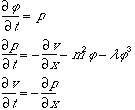
The choice of symbols p and v is inspired by acoustics. The acoustic wave equation looks a lot like the Klein Gordon equation.

Negative mass.

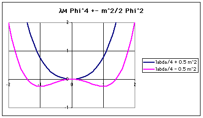
Normally, you don't use negative values of m^2, because it generates "runaway" solutions, that grow to infinite values with time. But the labda term can ensure the global stability of the equations, in spite of a negative mass. In the graph below the phi^x terms of the Lagrangian are plotted. The graph shows that in the negative mass case, the function has a local maximum, and 2 local minima. It turns out that the local maximum corresponds to an unstable equilibrium. 

The equation with negative mass is:
 

This equation is seen also in the so-called Higgs mechanism, which plays a role in the quantum theory of weak interactions.

Electric equivalent.

The equation is related to the electric circuit equivalent of the Klein Gordon equation.

Analytical solutions

When I first ran a simulation, which was with m=0, I noticed a soliton-like solution. (Click here for an introduction to solitons). I guessed the analytical form of the solution:

When you fill this in, you find:

A More general solution is:

A solution found in the literature is the so-called "kink" solution, which is:

This solution is only valid for negative mass, m^2 < 0.

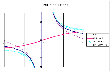
The kink solution looks quite different from the 1/r solution, as you fan see from the graph.

 
However, another solutions, related to the kink are:

(m^2 < 0)

(m^2 > 0)

(m^2 > 0)

These solutions are also in the graph. 

They look more like 1/r, and indeed approach 1/r in the limit for m->0.

The 1/r solution can be generalised to multi-dimensional waves:

Where D is the dimension of space. This means the solution is trivial for 3D space, because A=0. For D>3, A becomes imaginary. Formally this is a solution, but not for a real field phi. You could remedy this by letting labda be negative. However, that will generate "runaway" solutions that grow indefinately in magnitude with time.

Other solutions in higher dimensions are the lower dimensional solutions, but with zero gradient in the new dimensions. An interesting one is the 2D 1/r solution. It forms a longs cylinder, or string. It is conceivable that one could bend this string, whereby the string reacts elastically. This is interesting, because String Theory is a hot topic in Physics at the moment.

The equipartition Principle.

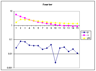
One of the reasons for doing this simulation, was a preparation for doing a quantum field simulation. Quantum mechanics is supposed to save us from the "UV catastrophe".

The UV catastrophe was the problem that Max Plank was working on when he proposed the first quantum theory. The principle of equipartition of energy supposes that all degrees of freedom have  average energy kT. For fields like thermal radiation this is in agreement with experiment for low frequencies. But the principle predicts that for UV, roentgen and gamma rays, you should also have kT per degree of freedom. That predicts a far too large amount of high frequency radiation. (Gamma rays were not yet discovered, I'm not sure about Roentgen, so they called the prediction the "UV-catastrophe") If you assume that energy comes in lumps of amount h*f, you get the right answer.

Maybe Plank guessed this by comparing a graph of (E vs. f) to a graph of (E vs. 0.5*mv^2) for atoms (i.e.. the Boltzman distribution). The Boltzman distribution for high energy is proportional to:
~exp (-(0,5mv^2)/kT)
This curve looks just like the observed curve for thermal radiation
~exp (-hf/kT)

By comparing:
v^2 <-> f
m    <-> h
You could speculate that Plank said "Hey, kinetic energy comes in lumps of m, and if radiation energy comes in lumps of h, it would just work out". Actually, I have been told that this is not the way Plank did it, but anyway.
 
 Before doing a quantum field simulation to see how it saves us from the UV catastrophe, I want to see the effect in classical physics. Because of the discrete grid, there is no problem with infinite energy as the energy can occupy unlimitedly small wavelengths. But still, the equipartition principle predicts that the frequency spectrum will be white. Quantum physics predicts that the frequency spectrum will have a drop-off ~exp (-hf/kT) .

But solitons can prevent the equipartition from happening. Actually, they are a bit "quantum"-like, because the amplitude of the solution is fixed.

I havent' figured out yet if the equipartition principle holds. I you initiate the simulation with a white spectrum ,it tends to stay white. If you initiate it with only low frequencies, they not *not* transfer energy to higher modes until equipartion. But maybe you get equipartition after you subtract away some soliton-like structures.

 
 
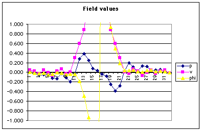
 Typical results